Given observed time series and a target time series of interest, can we identify the causes of the target, without excluding the presence of hidden time series? This question arises in many fields — such as finance, biology, and supply chain management — where sequences of data constitute partial observations of a system.
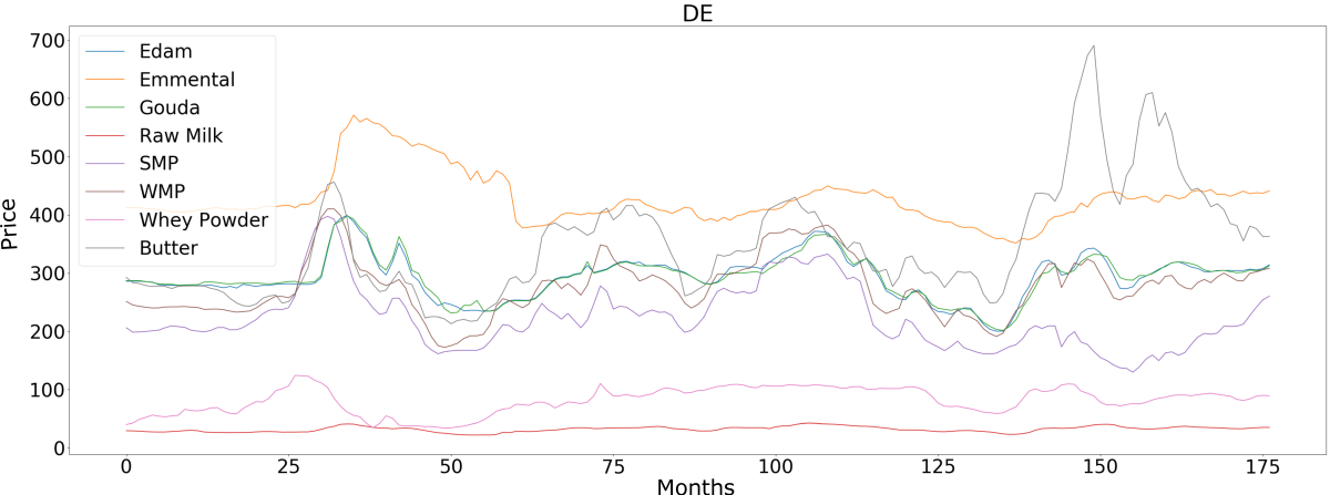
Imagine, for instance, that we have time series for the prices of dairy products. From the data alone, can we identify the causes of fluctuations in the price of butter?
The standard way to represent causal relationships between variables that are associated with each other is with a graph whose nodes represent variables and whose edges represent causal relationships.
In a paper that we presented at the International Conference on Machine Learning (ICML) 2021, coauthored by Bernhard Schölkopf, we described a new technique for detecting all the direct causal features of a target time series — and only the direct or indirect causal features — given some graph constraints. The proposed method yielded false-positive rates of detected causes close to zero.
The constraints we observe refer to the target and the “memory” of some hidden time series (the lack of dependency on their own pasts, in some cases). We wanted to limit our assumptions to those that can be naturally derived from the setting and that could not be avoided otherwise. Therefore, we wanted to avoid strong assumptions made by other methods, such as excluding hidden common causes (unobserved time series that caused multiple observed ones).
We also wanted to avoid other drawbacks of prior methods, such as requiring interventions on the system (to test for particular causal sequences) and requiring large conditioning sets (sets of variables that must be controlled for to detect dependences) or exhaustive conditional-independence tests, which hinder the statistical strength of the outcome.
Our method, by contrast, accounts for hidden common causes, uses only observational data, and constructs conditioning sets that are small and efficient in terms of signal-to-noise ratio, given some graph constraints that seemed hard to avoid.

Conditional independence
As is well known, statistical dependence (i.e., correlation in linear cases) does not imply causation. The graphs we use to represent causal relationships between associated variables are so-called directed acyclic graphs (DAGs), meaning the edges have direction and there are no loops. The direction of the edges (represented by arrows in the graphs below) indicates the direction of causal influence. In the time series case, we use “full time DAGs”, where each node represents a different time step from a time series.
To analyze whether a third variable, S, explains a statistical dependency (i.e., correlation) between two other variables, one checks whether the dependency disappears after restricting the statistics to data points with fixed values of S. In larger graphs, S can be a whole set of variables, which we call a conditioning set. Controlling for all the variables in a conditioning set is known as conditional independence testing and is the main tool we use in our method.
Another important notion is that of confounding. If two variables, X and Y, are dependent, not because one causes the other, but because they’re both caused by a third variable, U, we say that they are confounded by U.
Before we get into the complex graphs of time series, let's present the intuition behind our method with simple graphs.
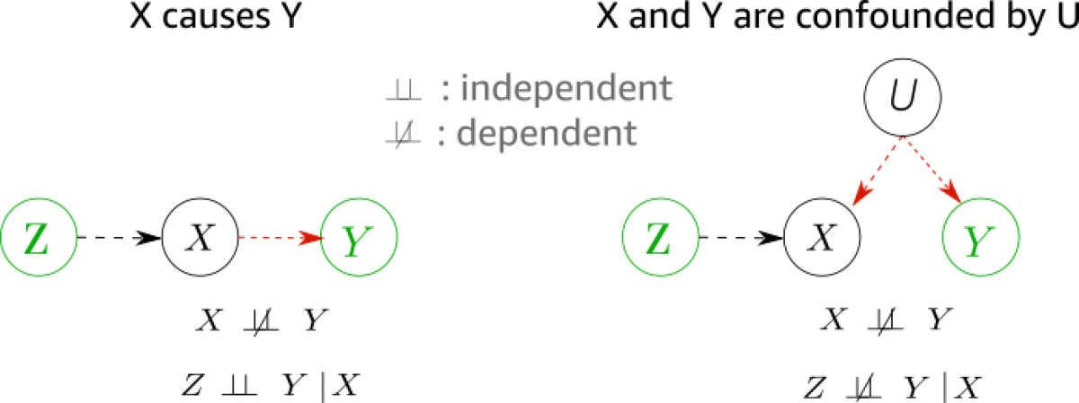
In the graphs below, we manage to distinguish between causal influence and confounding relationships by searching for different patterns of conditional independence. In both graphs, X and Y are dependent (i.e., they vary together). But in the left-hand graph, Z and Y are independent when we condition on the cause X; i.e., when we control for X, variations in Y become independent from variations in Z.
When, however, there is a hidden confounder between X and Y, as in the graph at right, Z and Y become dependent when conditioning on X.
This can seem counterintuitive. When we condition on a variable, we treat it as if we know its outcome. In the graph below, because we know how Z contributes to X, the difference between this contribution and the actual value of X comes from U (with some variation from noise). Since Y varies with U, it reflects that variation as well, and Z and Y become dependent.
Causality in time series
This idea of finding similar characteristic patterns of conditional independences to distinguish causes from confounders is very relevant to our method. In the time series case, the graph is much more complicated than in the examples above. Here we show such a time series graph:
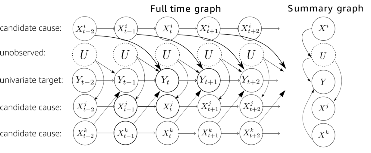
Here, we have a univariate (one-dimensional) target time series, Y, whose causes we want to find. Then we have several observed candidate time series, Xi, which might be causing the target or have different dependencies with it. Finally, we allow for the existence of several hidden time series, U.
We know the directions of some edges from the time order, which is helpful. On the other hand, time series’ dependence on their own pasts complicates the picture, because it creates common-cause schemes between nodes.
For each candidate time series, we want to isolate the current and previous node and the corresponding target node. We thus extract triplets like the one indicated by green and yellow in the graph below.
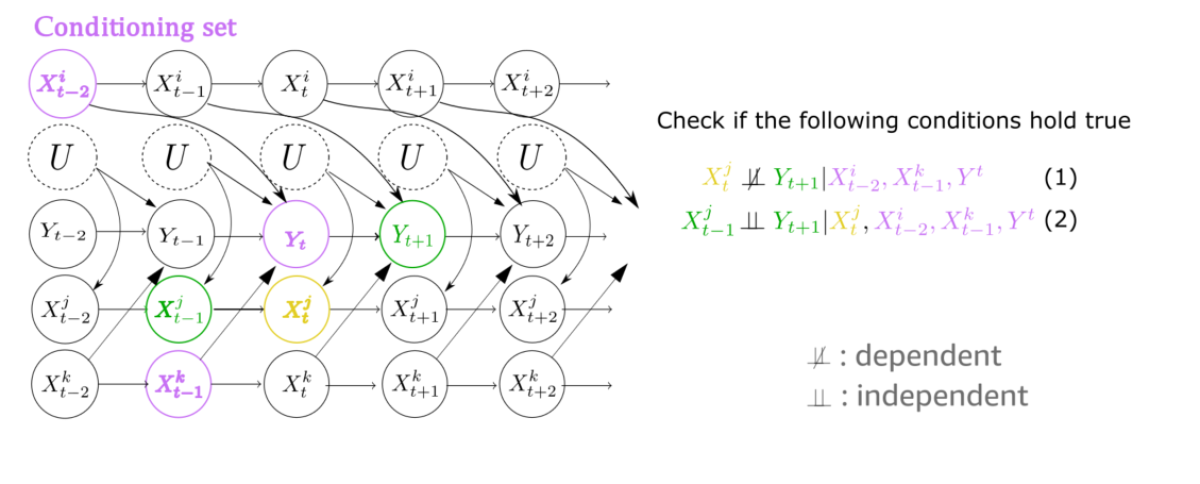
If we manage to do that, then it is enough to check whether the green nodes become independent when we simultaneously condition on the yellow node and all the purple ones.
If there is a hidden confounder between the yellow node and the target’s green node, then, conditioning on the yellow node will force a dependence between the two green nodes, as in the first example above. But to perform that test, we need to isolate our triplet from the causal influences of other time series.
To do that, we construct a conditioning set, S, that includes at most one node from each time series that is dependent on the target. This node corresponds to the one that enters the previous time stamp of the target (Yt in the graph above). And of course, we also need to include the previous time stamp of the target node itself (Yt, above) to remove the target's past dependency, as well as the yellow node.
Here we see that indeed the relationship between Xj and Y is confounded (Xj does not cause Y, although they appear to be related). We see that the second condition of our method is violated, and consequently, Xj is correctly rejected (as it is not a cause of Y).
Given some restrictions on the graph, which we do not consider extreme given the hardness of hidden confounding, we propose and prove two theorems for the identification of direct and indirect causes in single-lag graphs — that is, graphs in which a node in a candidate time series shares only one edge with nodes in the target time series. These theorems result in an algorithm with only two conditional-independence tests and well-defined conditioning sets, which scales linearly with the number of candidate time series.

We now return to our original motivational example, predicting the price of butter. The real-world data we used to test our approach included the price of raw milk, the price of butter, and, depending on the country, the prices of other dairy products, such as cheese and whey powder. Our method correctly deduced that the price of butter was caused by the price of raw milk but not by the prices of other dairy products, although they were strongly dependent on it. In one dataset, where the data did not include the price of raw milk, our method correctly deduced that the dependencies between the price of butter and the prices of other dairy products did not imply causation.


