An automatic-speech-recognition system — such as Alexa’s — converts speech into text, and one of its key components is its language model. Given a sequence of words, the language model computes the probability that any given word is the next one.
For instance, a language model would predict that a sentence that begins “Toni Morrison won the Nobel” is more likely to conclude “Prize” than “dries”. Language models can thus help decide between competing interpretations of the same acoustic information.
Conventional language models are n-gram based, meaning that they model the probability of the next word given the past n-1 words. (N is typically around four.) But this approach can miss longer-range dependencies between words: for instance, sentences beginning with the phrase “Toni Morrison” may have a high probability of including the phrase “Nobel Prize”, even if the two phrases are more than four words apart.
Recurrent neural networks can learn such long-range dependencies, and they represent words as points in a continuous space, which makes it easier to factor in similarities between words. But they’re difficult to integrate into real-time speech recognition systems. In addition, although they outperform conventional n-gram-based language models, they have trouble incorporating data from multiple data sets, which is often necessary, as data can be scarce in any given application context.
In a paper we’re presenting at Interspeech, my colleagues and I describe a battery of techniques we used to make neural language models practical for real-time speech recognition. In tests comparing our neural model to a conventional model, we found that it reduced the word recognition error rate by 6.2%.
In our experiments, we investigated the scenario in which in-domain data is scarce, so it has to be supplemented with data from other domains. This can be tricky. After all, language models are highly context dependent: the probabilities of the phrases “Red Sox” and “red sauce”, for instance, would be very different in the sports domain and the recipe domain.
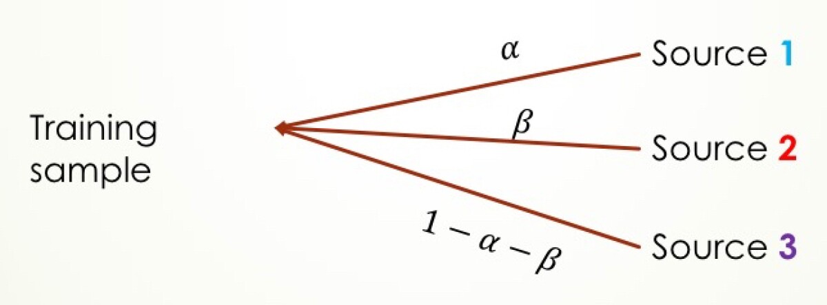
To ensure that we were using data from other domains effectively, we first built conventional n-gram language models for our in-domain and out-of-domain training data sets. These models were combined linearly to minimize perplexity — a measure of how well a probability distribution predicts a sample — on in-domain data. On the basis of this, we assigned each data set a score that measured its relevance to the in-domain data.
That score then determined the likelihood that a sample from a given data set would be selected for the supplementary data set. If, for instance, the in-domain data set had a relevance score of 75%, and a second out-of-domain data set had a score of 25%, then the first set would contribute three times as many samples to the training data as the second.

We combined this novel data-sampling strategy with transfer learning, by initializing our model’s parameters on out-of-domain data.
This addressed the data scarcity problem, but we still had to contend with the challenge of integrating neural networks into the speech recognizer without adding much additional latency to the system. Our approach was one that’s common in neural-language-model research: we begin by passing incoming data through a speech recognizer with a conventional n-gram language model, then refine the first model’s hypotheses using the neural model.
The risk with this approach is that the n-gram model will reject hypotheses that the more powerful neural model would find reason to consider. To lower that risk, once we had built our neural model, we used it to generate synthetic data, which provided supplementary training data for the first-pass model. This brought the two models into better alignment.
Taking advantage of the two-pass approach also required some changes to the way we trained our neural model. Typically, a neural language model that had been fed a sequence of words would compute the probability that every word in its vocabulary should be the next word. Once you factor in names like Toni Morrison’s, a speech recognition application could easily have a vocabulary of a million words, and computing a million separate probabilities for every input would be time consuming.
The first-pass model, however, should have winnowed the number of possibilities down to just a handful, and we wanted our neural model to consider only those possibilities. So we trained it using a technique called noise contrastive estimation.
When a recurrent language model is fed a sentence, it processes the words of the sentence one at a time. That’s how it learns to model dependencies across sequences of words.
With noise contrastive estimation, the model is trained on pairs of words, not individual words. One of the paired words is the true target — the word that actually occurs at that position in the input sentence. The other word is randomly selected, and the model must learn to tell the difference. At training time, this turns the task of computing, say, a million probabilities into a simple binary choice. Moreover, at inference time, the model can directly estimate the probability of the target word, without normalizing over all of the other words in the vocabulary, thus drastically reducing the computational cost.
Finally, to increase the efficiency of our neural model still further, we quantize its weights. A neural network consists of simple processing nodes, each of which receives data from several other nodes and passes data to several more. Connections between nodes have associated weights, which indicate how big a role the outputs of one node play in the computation performed by the next.
Quantization is the process of considering the full range of values that a particular variable can take on and splitting it into a fixed number of intervals. All the values within a given interval are then approximated by a single number.
Quantization makes the neural language model more efficient at run time. In our experiments, the addition of the neural model increased processing time by no more than 65 milliseconds in 50% of cases and no more than 285 milliseconds in 90% of cases, while reducing the error rate by 6.2%.
Acknowledgments: Denis Filimonov, Gautam Tiwari, Guitang Lan, Ariya Rastrow


