Historically, Alexa’s automatic-speech-recognition models, which convert speech to text, have run in the cloud. But in recent years, we’ve been working to move more of Alexa’s computational capacity to the edge of the network — to Alexa-enabled devices themselves.
The move to the edge promises faster response times, since data doesn’t have to travel to and from the cloud; lower consumption of Internet bandwidth, which is important in some applications; and availability on devices with inconsistent Internet connections, such as Alexa-enabled in-car sound systems.
At this year’s Interspeech, we and our colleagues presented two papers describing some of the innovations we’re introducing to make it practical to run Alexa at the edge.
In one paper, “Amortized neural networks for low-latency speech recognition”, we show how to reduce the computational cost of neural-network-based automatic speech recognition (ASR) by 45% with no loss in accuracy. Our method also has lower latencies than similar methods for reducing computation, meaning that it enables Alexa to respond more quickly to customer requests.
In the other paper, “Learning a neural diff for speech models”, we show how to dramatically reduce the bandwidth required to update neural models on the edge. Instead of transmitting a complete model, we transmit a set of updates for some select parameters. In our experiments, this reduced the size of the update by as much as 98% with negligible effect on model accuracy.
Amortized neural networks
Neural ASR models are usually encoder-decoder models. The input to the encoder is a sequence of short speech snippets called frames, which the encoder converts into a representation that’s useful for decoding. The decoder translates that representation into text.
Neural encoders can be massive, requiring millions of computations for each input. But much of a speech signal is uninformative, consisting of pauses between syllables or redundant sounds. Passing uninformative frames through a huge encoder is just wasted computation.
Our approach is to use multiple encoders, of differing complexity, and decide on the fly which should handle a given frame of speech. That decision is made by a small neural network called an arbitrator, which must process every input frame before it’s encoded. The arbitrator adds some computational overhead to the process, but the time savings from using a leaner encoder is more than enough to offset it.
Researchers have tried similar approaches in domains other than speech, but when they trained their models, they minimized the average complexity of the frame-encoding process. That leaves open the possibility that the last few frames of the signal may pass to the more complex encoder, causing delays (increasing latency).
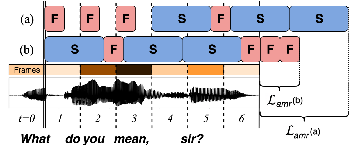
In our paper, we propose a new loss function that adds a penalty (Lamr in the figure above) for routing frames to the fast encoder when we don’t have a significant audio backlog. Without the penalty term, our branched-encoder model reduces latency to 29 to 234 milliseconds, versus thousands of milliseconds for models with a single encoder. But adding the penalty term cuts latency even further, to the 2-to-9-millisecond range.

In our experiments, we used two encoders, one complex and one lean, although in principle, our approach could generalize to larger numbers of encoders.
We train the arbitrator and both encoders together, end to end. During training, the same input passes through both encoders, and based on the accuracy of the resulting speech transcription, the arbitrator learns a probability distribution, which describes how often it should route frames with certain characteristics to the slow or fast encoder.
Over multiple epochs — multiple passes through the training data — we turn up the “temperature” on the arbitrator, skewing the distribution it learns more dramatically. In the first epoch, the split for a certain type of frame might be 70%-30% toward one encoder or the other. After three or four epochs, however, all of the splits are more like 99.99%-0.01% — essentially binary classifications.
We used three baselines in our experiments, all of which were single-encoder models. One was the full-parameter model, and the other two were compressed versions of the same model. One of these was compressed through sparsification (pruning of nonessential network weights), the other through matrix factorization (decomposing the model’s weight matrix into two smaller matrices that are multiplied together).
Against the baselines, we compared two versions of our model, which were compressed through the same two methods. We ran all the models on a single-threaded processor at 650 million FLOPs per second.
Our sparse model had the lowest latency —two milliseconds, compared to 3,410 to 6,154 milliseconds for the baselines — and our matrix factorization model required the fewest number of floating-point operations per frame — 23 million, versus 30 million to 43 million for the baselines. Our accuracy remained comparable, however — a word error rate of 8.6% to 8.7%, versus 8.5% to 8.7% for the baselines.
Neural diffs
The ASR models that power Alexa are constantly being updated. During the Olympics, for instance, we anticipated a large spike in requests that used words like “Ledecky” and “Kalisz” and updated our models accordingly.
With cloud-based ASR, when we’ve updated a model, we simply send copies of it to a handful of servers in a data center. But with edge ASR, we may ultimately need to send updates to millions of devices simultaneously. So one of our research goals is to minimize the bandwidth requirements for edge updates.
In our other Interspeech paper, we borrow an idea from software engineering — that of the diff, or a file that charts the differences between the previous version of a codebase and the current one.
Our idea was that, if we could develop the equivalent of a diff for neural networks, we could use it to update on-device ASR models, rather than having to transmit all the parameters of a complete network with every update.
We experimented with two different approaches to creating a diff, matrix sparsification and hashing. With matrix sparsification we begin with two matrices of the same size, one that represents the weights of the connections in the existing ASR model and one that’s all zeroes.
Then, when we retrain the ASR model on new data, we update, not the parameters of the old model, but the entries in the second matrix — the diff. The updated model is a linear combination of the original weights and the values in the diff.
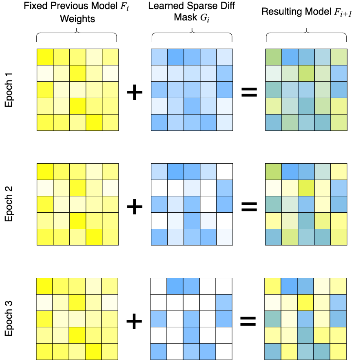
When training the diff, we use an iterative procedure that prunes matrices with too many non-zero entries. As we did when training the arbitrator in the branched-encoder network, we turn up the temperature over successive epochs to make the diff sparser and sparser.
Our other approach to creating diffs was to use a hash function, a function that maps a large number of mathematical objects to a much smaller number of storage locations, or “buckets”. Hash functions are designed to distribute objects evenly across buckets, regardless of the objects’ values.
With this approach, we hash the locations in the diff matrix to buckets, and then, during training, we update the values in the buckets, rather than the values in the matrices. Since each bucket corresponds to multiple locations in the diff matrix, this reduces the amount of data we need to transfer to update a model.
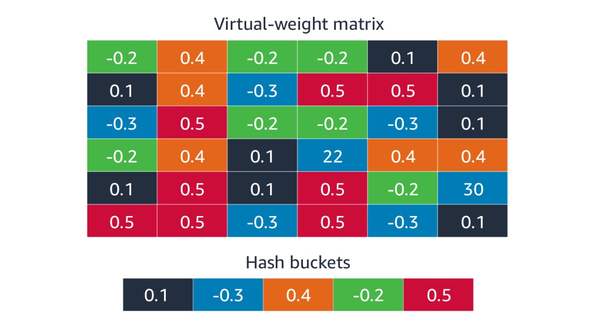
One of the advantages of our approach, relative to other approaches to compression, such as matrix factorization, is that with each update, our diffs can target a different set of model weights. By contrast, traditional compression methods will typically lock you into modifying the same set of high-importance weights with each update.

In our experiments, we investigated the effects of three to five consecutive model updates, using different diffs for each. Hash diffing sometimes worked better for the first few updates, but over repeated iterations, models updated through hash diffing diverged more from full-parameter models. With sparsification diffing, the word error rate of a model updated five times in a row was less than 1% away from that of the full-parameter model, with diffs whose size was set at 10% of the full model’s.


