Commercial machine learning systems are trained on examples meant to represent the real world. But the world is constantly changing, and deployed machine learning systems need to be regularly reevaluated, to ensure that their performance hasn’t declined.
Evaluating a deployed AI system means manually annotating data the system has classified, to determine whether those classifications are accurate. But annotation is labor intensive, so it is desirable to minimize the number of samples required to assess the system’s performance.
Many commercial machine learning systems are in fact ensembles of binary classifiers; each classifier “votes” on whether an input belongs to a particular class, and the votes are pooled to produce a final decision.
In a paper we’re presenting at the European Conference on Machine Learning, we show how to reduce the number of random samples required to evaluate ensembles of binary classifiers by exploiting overlaps between the sample sets used to evaluate the individual components.
For example, imagine that an ensemble that has three classifiers, and we need 10 samples each to evaluate the performance of the three classifiers. Evaluating the ensemble requires 40 samples — 10 each for the individual classifiers and 10 for the full ensemble. If 10 of the 40 samples were duplicates, we could make do with 30 annotations. Our paper builds on this intuition.
In an experiment using real data, our approach reduced the number of samples required to evaluate an ensemble by more than 89%, while preserving the accuracy of the evaluation.
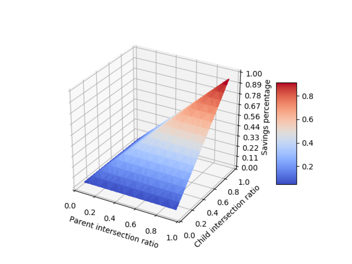
We also ran experiments using simulated data that varied the degree of overlap between the sample sets for the individual classifiers. In those experiments, the savings averaged 33%.
Finally, in the paper, we show that our sampling procedure doesn’t introduce any biases into the resulting sample sets, relative to random sampling.
Common ground
Intuitively, randomly chosen samples for the separate components of an ensemble would inevitably include some duplicates. Most of the samples useful for evaluating one model should thus be useful for evaluating the others. The goal is to add in just enough additional samples to be able to evaluate all the models.
We begin by choosing a sample set for the entire ensemble, which we dub the “parent”; the individual models of the ensemble are, by reference, “children”. After finding a set of samples sufficient for evaluating the parent, we expand it to include the first child, then repeat the procedure until the set of samples covers all the children.
Our general approach works with any criterion for evaluating an ensemble’s performance, but in the paper, we use precision — or the percentage of true positives that the classifier correctly identifies — as a running example.

We begin with the total set of inputs that the parent has judged to belong to the target class and the total set of inputs that the child has. There’s usually considerable overlap between the two sets; for example, in a majority-vote ensemble composed of three classifiers, the ensemble (parent) classifies an input as positive as long as two of the components (children) do.
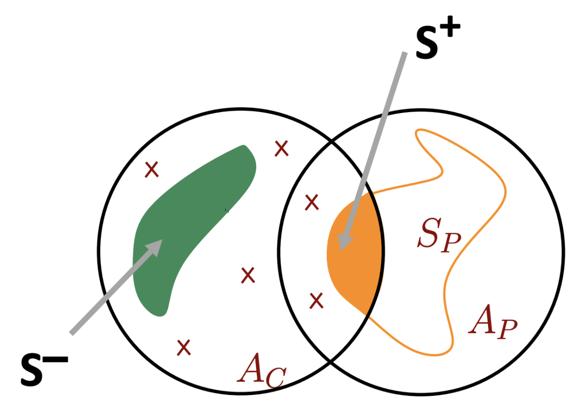
From the parent set, we select enough random samples to evaluate the parent. Then we find the intersection between that sample set and the child’s total set of positive classifications (S+ in the figure above). This becomes our baseline sample set for the child.
Next, we draw a random sampling of inputs that the child classified as positive but the parent did not (S-, above). The ratio between the size of this sample and the size of the baseline sample set should be the same as the ratio between the number of inputs that the child — but not the parent — labeled positive and the number of inputs that both labeled positive.
When we add these samples to the baseline sample set, we get a combined sample set that may not be large enough to accurately estimate precision. If needed, we select more samples from the inputs classified as positive by the child. These samples may also have been classified as positive by the parent (Sremain in the figure above).
Recall that we first selected samples from the set where the child and parent agreed, then from the set where the child and parent disagreed. That means that the sample set we have constructed is not truly random, so the next step is to mix together the samples in the combined set.
Reshuffle or resample?
We experimented with two different ways of performing this mixing. In one, we simply reshuffle all the samples in the combined set. In the other, we randomly draw samples from the combined set and add them to a new mixed set, until the mixed set is the same size as the combined set. In both approaches, the end result is that when we pick any element from the sample, we won’t know whether it came from the set where the parent and child agreed or the one where they disagreed.

In our experiments, we identified a slight trade-off between the results of our algorithm when we used reshuffling to produce the mixed sample set and when we used resampling. Because resampling introduces some redundancies into the mixed set, it requires fewer samples than reshuffling, which increases the savings in sample size versus random sampling.
At the same time, however, it slightly lowers the accuracy of the precision estimate. With reshuffling, our algorithm, on average, slightly outperformed random sampling on our three test data sets, while with resampling, it was slightly less accurate than random sampling.
Overall, the sampling procedure we have developed reduces the sample size. Of course, the amount of savings depends on the overlap between the parent’s and child’s judgments. The greater the overlap, the greater the savings in samples.


