When football fans evaluate a player’s performance, they measure the player’s execution of specific plays against an innate sense of the player’s potential. Trying to encode such judgments into machine learning models, however, has proved non-trivial.
Fans and commentators have criticized existing quarterback (QB) passing stats, such as Madden QB, the NFL passer rating, ESPN’s total quarterback rating (QBR), and the Pro Football Focus (PFF) grade, for being calibrated to obsolete data, being unrelated to winning, or scoring players anomalously — as when Kyler Murray received the low Madden QB21 rating of 77 despite being the 2019 Offensive Rookie of the Year.
On January 13, 2022, just before Super Bowl LVI, the NFL announced its new QB passing score, which seeks to improve on its predecessors’ limitations and to isolate a QB’s contributions from those of the team in a completely data-driven way.
The play level
A root problem with existing ratings is their inconsistency across plays, games, weeks, and seasons. We sought a metric that could account for play-specific dynamics and scale to different granularities with consistency.
We wanted to measure the QB’s decision making and pass execution given the game clock and the pressure he was under. For those conditions, we have directly measurable quantities, such as the defense’s movements. But how do we measure how “well” the QB performed? This is a point we address in the next section (“The model architecture”), but for now, we take yards gained as a measurable outcome. (This assumption will prove useful downstream.)
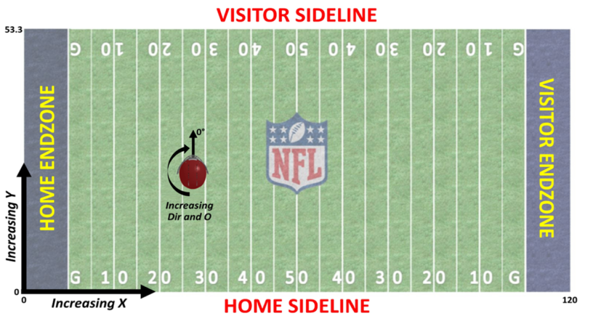
Since we said we wanted to take a data-driven approach, let’s look at exactly what the data is.
On each play, we receive updates every 100 milliseconds from radio frequency ID chips in the players’ shoulder pads, giving us all 22 players’ position in the (x, y)-coordinates of the field, along with their speed, acceleration, running direction, and body orientation, as shown in the image above.
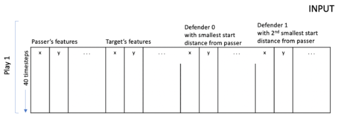
This time series is of variable length, starting with the snap and ending when the QB releases the ball. For example, a QB throwing four seconds after the snap yields a time series of 40 timesteps, whereas a pass that takes just over two seconds yields a time series of 25 timesteps.
The figure below shows how the time series is represented. Each row corresponds to a single timestep and contains eight features (x-position, y-position, x-speed, y-speed, x-acceleration, y-acceleration, direction, and orientation) for each of 22 players, for a matrix of 176 columns and 40 rows. Features such as the number of defenders within a two-yard radius of the target receiver receive additional columns, but we eschew them here to focus on modeling technique.
The collection of passing plays from the 2018-2020 seasons provided us with around 34,000 completions, 15,000 incompletes, and 1,200 interceptions, for more than 50,000 plays total. Feature preprocessing is a memory-intensive job, requiring two hours runtime on a ml.m5.m24xlarge instance. Modeling so large a number of time series, however, is a high-compute job.
For the model described in the upcoming section, the one-gpu p3.8xlarge instance incurred an eight-hour training time. While the NFL can afford two-hour preprocessing and eight-hour model fittings before the season commences, in live televised games, the inference returning a QB’s score for his play needs to be in real-time, like the 0.001 second per play of the following model.
The model architecture
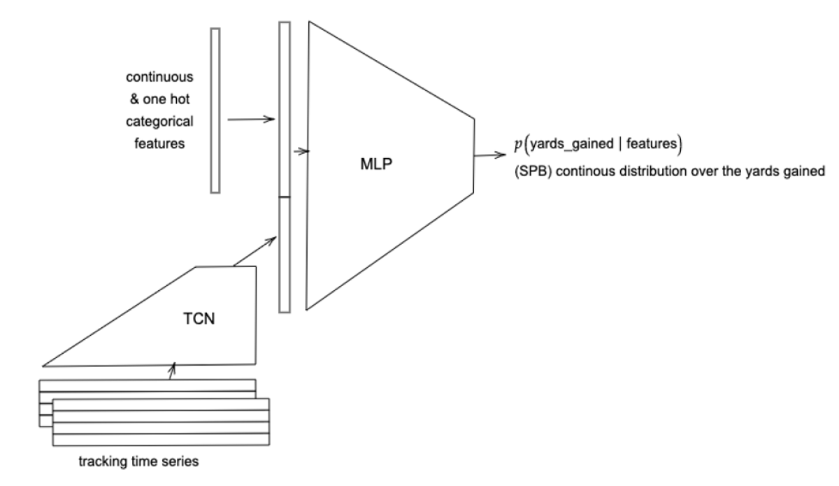
To learn the temporal complexities within plays’ time series, we opted for a temporal convolutional network (TCN), a convolutional network adapted to handle inputs of different lengths and factor in long-range relationships between sequential inputs.
Since a play also has static attributes — such as down, score, and games remaining in the season — that influence players’ decisions and performance, we concatenate these with the TCN state and pass both to a multilayer perceptron to produce the final output, a probabilistic prediction of yards gained. To that, we compare the play’s actual yards gained.
Now, the network output is worth careful consideration. Naively, one might want to output a point prediction of the yards gained and train the network with an error loss function. But this fails to achieve the desired goal of measuring the outcome of a play relative to its potential.
An extra two yards gained under easier circumstances is not the same as two yards gained in more difficult circumstances, yet both would have a mean absolute error (MAE) of two yards. Instead, we opted for a distributional prediction, where the network’s outputs are parameters that specify a probability distribution.
We thought about which probability distribution function (PDF) would be most suitable. For certain plays, the PDF of yards gained would need to be asymmetrical: e.g., in a completed pass, if the QB throws to a receiver already running toward the end zone, positive yards gained are more likely than negative yards. Whereas for other plays, the PDF of yards gained would need to capture symmetry: on an interception, for example, the “negative” yards gained by the defender would balance against the possible positive yards gained by a completion.
There are even those plays for which the PDF would be bimodal: if the QB passes to a receiver with only one defender closing in, then the likelihood of yards gained lies either in the one- to two-yards range (if the receiver is tackled) or in the high-yardage range (if the receiver eludes the tackle), but not in-between. Other multi-model plays include when the QB may have to scramble for yards, like in the second play in this video.
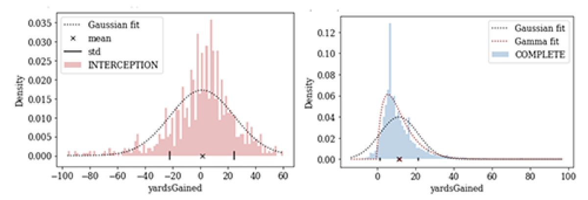
So we needed a distribution whose parameterization is flexible enough to accommodate multimodality, different symmetries, and light or heavy tails and whose locations and scale can vary with the clock time, current score, and other factors. We can’t meet these requirements with distributions like Gaussian or gamma, but we can meet them with the spliced binned-Pareto distribution.
The spliced binned-Pareto distribution
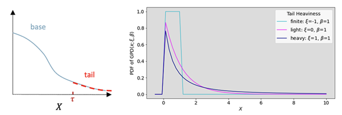
The spliced binned-Pareto (SBP) distribution arises from a classic result in extreme-value theory (EVT), which states that the distribution of extreme values (i.e., the tail) is almost independent of the base distribution of the data and, as shown below, can be estimated from the datapoints above the assumed upper bound (t) of the base distribution.
The second theorem of EVT states that any such distribution tail can be well-approximated by a generalized Pareto distribution (GPD) that has only two parameters, shape (x) and scale (b), and closed-form quantiles. The figure below shows the PDF of a GPD for x < 0, yielding a finite tail; x = 0, yielding an exponential tail; and x > 0, yielding a heavier-than-exponential tail.
Since we need multimodality and asymmetry for the base distribution, we modeled the base of the predictive distribution with a discrete binned distribution; as shown below, we discretize the real axis between two points into bins and predict the probability of the observation falling in each of these bins.
This yields a distribution robust to extreme values at training time because it is now a classification problem. The log-likelihood is not affected by the distance between the predicted mean and the observed point, as would be the case when using a Gaussian, Student’s t, or other parametric distribution. Moreover, the bins’ probability heights are independent of one another, so they can capture asymmetries or multiple modes in the distribution.
From the binned distribution, we delimit the lower tail by the fifth quantile and replace it with a weighted GPD. Analogously, we delimit the upper tail by the 95th quantile and replace it with another weighted GPD, to yield the SBP shown below.

The figure on the left above shows that the base distribution is indeed robust: the event represented by the extreme red dot will not bias the learned mean of the distribution but simply inflate the probability associated with the far-right bin.
However, this still leaves two problems: (i) although the red-dot event was observed to occur, the binned distribution would give it zero probability; conversely, (ii) the distribution would predict with certainty that extreme (i.e., great) plays do not occur. Because extreme yardage from deep-pass touchdowns, breakaway interceptions, etc., is rare, it is the adrenaline of the sport and exactly what we are most interested in describing probabilistically. The SBP figure above on the right graphically illustrates how the GPD tails can quantify how much less likely — i.e., harder — each incremental yard is.
The binned distribution and the GPDs are parameterized by the neural network we described above, which takes as input play matrices and outputs parameters: each of the bin probabilities, as well as x and b for each of the GPDs, which can be used to predict the probability-of-yards-gained value.
Establishing a gradient-based learning of heavy-tailed distributions has been a challenge in the ML community. Carreau and Bengio’s Hybrid Pareto model stitched GPD tails onto parametric distributions, but since the likelihood isn’t differentiable with respect to the threshold t, their model is supplemented with simulation and numerical approximations, foregoing time-varying applications. Other previous methods such as SPOT, DSPOT, and NN-SPOT, forego modeling the base and capture only the tails outside a fixed distance from the mean, which precludes higher-order non-stationarity and asymmetric tails.
While prior methods use a fixed threshold t to delimit tails, by modeling the base distribution, we obtain a time-varying threshold. Furthermore, training a single neural network to maximize the log-probability of the observed time step under the binned and GPD distributions yields a prediction that accounts for temporal variation in all moments of the distribution — the mean and variance as well as tail heaviness and scale, including asymmetric tails. The capabilities of different approaches are tabled below.

While we need a distributional prediction to grade a QB’s performance — to compare our model’s accuracy to other models’ — we need to use point predictions of yards gained. The table below compares the MAE of our method’s predictive median against that of a neural network with Gaussian output and against the point prediction of XGBoost, a decision-tree-based model.

We have released Pytorch code for the spliced binned-Pareto model, along with a demo notebook.
The NGS passing score
Our model’s predictive PDF quantifies how likely each yardage gain is, for a league-average QB, given a specific play’s circumstances. Therefore, evaluating the actual yards gained in the cumulative distribution function (CDF) of that play’s SBP distribution yields a ranking between 0 and 1 of that QB’s performance relative to peer QBs.
This CDF ranking, under some further standardizations, becomes the QB passing score at the play level.
Aggregating scores over multiple plays yields game-, season-, or other split-level QB passing scores. For example, based on all targeted pass attempts in the ’21 season, Kyler Murray has a score of 87, ranking him ninth out of playoff QBs.
Under pressure, Murray's score jumps to 89; zooming in to passes between 2.5 and 4 seconds (in 2020 and 2021), Murray now scores a 99 in a five-way tie for the highest possible score. Other splits can also be contextualized with the NGS passing score, like deep passes, for example.
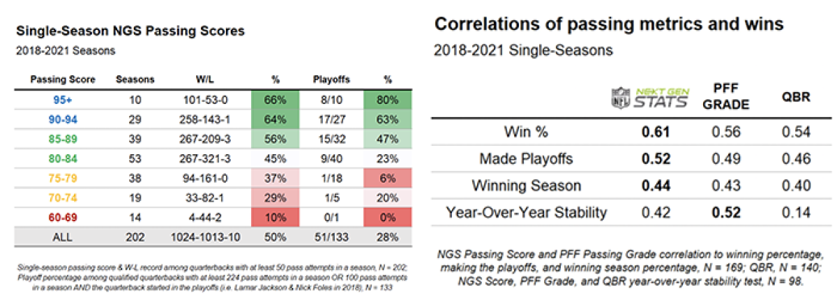
Finally, the tables below show that the NGS passing score correlates better with win percentages and playoff percentages than preceding passing metrics.
Acknowledgments: Brad Gross


